joint representative deep learning in heterogeneous graphs (september 2025)


robert hoang
project repositorypreface
Over the last two and a half weeks I lost sleep, appetite, and a fair amount of sanity studying classical and modern graph neural networks. What began as a single ChatGPT prompt spiraled into a few too many unplanned dates with equations I didn't recognize, papers I couldn't follow, and code that refused to run.
Everything that follows is the oversimplified aftermath.
abstract
Graph neural networks (GNNs) provide a framework for learning on non-Euclidean relational data, enabling pattern recognition in domains where structure is not easily observable (at least not to me). This work examines two algorithmic approaches to message passing in heterogenous graphs: node-only updates and joint node–edge updates. This project presents both an intuitive perspective and a linear algebraic formulation of these update rules, followed by empirical evaluation on heterogeneous transaction data.
My experiments highlight the tradeoffs between the simplicity of node-only updates and the additional expressivity gained by incorporating edge features. Results show that edge-aware updates can improve predictive performance in certain settings, though at the cost of increased complexity. Beyond performance metrics, this paper reflects on the mathematical intuition of the update rules and their implications for learning in heterogeneous graph structures.
introduction
GNNs extend deep learning to non-Euclidean data structures, where data is organized into nodes and edges rather than arrays or sequences like tabular data. By combining node features with relational information, GNNs have achieved strong results in applications such as fraud detection, recommender systems, drug discovery, and social network analysis.
Despite their success, the choice of update rules within a GNN remains an area of active research. Many models rely solely on node updates, treating edges as fixed carriers of connectivity, while others explicitly incorporate edge features into the update process. This design choice influences both the expressive power of the model and its computational complexity.
In this work, I examine and compare two approaches to message passing in bipartite graphs: node-only updates and joint node–edge updates. My goal is not only to evaluate their performance on 24 million points of transactional data and 4 million points of social network data, but also to highlight the trade-offs between simplicity and expressivity, and to provide a personal record of what I learned while experimenting with different update rules in GNNs.
background
Graphs represent data where relationships can often matter as much as the entities themselves. In a heterogenous graph, nodes are split into multiple classes with edges connecting across sets. More generally, heterogeneous graphs allow multiple node and edge types, capturing richer relational structures.
GNNs extend deep learning to these settings through message passing: nodes collect information from their neighbors, aggregate it, and update their state. The rule looks like this:

A node “listens” to its neighbors, compresses what it hears, and transforms that into a new representation. Classic models like GCN discovered by Kipf & Welling in 2017 (what we will be using), GraphSAGE (Hamilton et al., 2017), and GAT (Velickovic et al., 2018) refined this idea for scalability and attention. Later, models such as R-GCN, HAN, and HGT extended GNNs to heterogeneous graphs. More recent work also explores edge-aware updates, where edges carry features or even learn their own embeddings — an important idea for domains like recommendation or fraud detection.
node updating process
What follows is an oversimplified explanation of the mathematical process underlying a GNN forward pass.
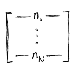
Assume you already have a sampled subgraph with feature matrix
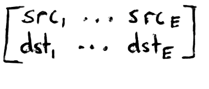
and an edge index matrix of the forms
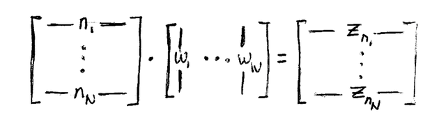
In one layer, you first apply a linear transformation to get source and destination embeddings.
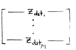
Then, for each destination node, you gather all incoming source embeddings into source and destination matrices and perform a segmented reduction to aggregate them.

Finally, you concatenate the aggregated neighbor embedding with the node's own transformed embedding and apply a non-linearity typically following this formula. Note that hj and hkare some combination (typically concatenation) of a node's source or destination embeddings on a directed graph.
or more formally
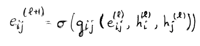
edge updating process
For each edge e = i → j, we construct a combined representation from the source node, destination node, and edge features. We then apply a non-linearity to get the updated edge embedding.
experiments
I initially began with IBM's fraud dataset, which contained over 24 million transactions across 100,000 merchants and 2,000 users. At first, I thought this dataset would be ideal, but I quickly found that the class prevalence was only 0.12% which made it extremely difficult to train without over sampling. I spent hours preprocessing and hand-building a full edge index, resulting in a graph that took up nearly 8 GB of space and required hours of training per run. Ultimately, the model underperformed badly. Structural anomalies weren't the real signal in this dataset — most fraud could be picked up with a simple multilayer perceptron using the raw features alone, making a graph-based approach unnecessary overhead.
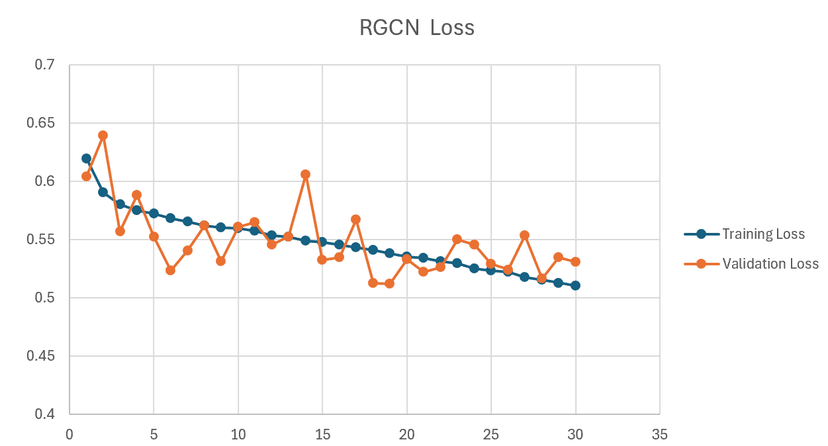
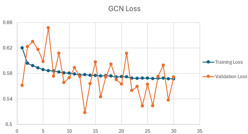
Given this, I shifted focus to the DGraph dataset which consisted of only 4 million edges with 3 million nodes (still not great numbers for structural anomalies but whatever), which targets fraudulent users on a fintech platform. Unlike IBM's dataset, this one was smaller, better structured, and already came with an edge index and useful preprocessing. I designed experiments to compare a vanilla GCN against a Relational GCN (RGCN) to evaluate whether explicitly modeling edge types and relationships meaningfully improved performance.
At this point, practicality mattered more than exhaustive optimization given that I expected the project to finish a week earlier. I therefore limited training to ~30 minutes per model with simple, untuned GCN and RGCN architectures in PyTorch Geometric. Using a patience of 10, both models reached a relatively flat loss curve. The RGCN outperformed the vanilla GCN in accuracy by 5% and by 4% in recall, which looks marginal but can actually represent a meaningful jump in real-world anomaly detection systems.

explanation
The RGCN outperformed the vanilla GCN primarily because it can model different relation types explicitly, rather than treating all edges as homogeneous. In relational data, the kind of interaction between nodes (e.g., collaboration, communication, or ownership) often carries more signal than the mere presence of a connection. In some sense, it's kind of like how the interactions between people carry more information about their relationship than their individual traits.
By separating these interactions, RGCNs can capture patterns that a GCN would not. However, since the DGraph dataset included very limited edge features, the benefit here seemed to be marginal, and the performance gap could have been much larger on a richer graph.
conclusion
Even though the models I built are far from perfect and by no means close to industry standard, this project taught me a lot. Just two weeks and a half ago I didn't know anything about GNNs, GCNs, RGCNs, or that they even existed, and now I've gone through the process of preprocessing and building graphs, sampling subgraphs, updating nodes and edges, and comparing their effects in practice.
The world is built on relationships, and I believe that graph neural networks are one step toward capturing them. I think that Bertalanffy said it best:
“The whole is more than the sum of its parts, not in an ultimate, metaphysical sense, but in the important pragmatic sense that the parts are shaped by the relations in which they stand.”
Thank you for reading.